作者:MARCIN ZABŁOCKI
编译:ronghuaiyang
导读
如何使用SimCLR框架进行对比学习,看这个就明白了。
在过去的几个月中,NLP和计算机视觉的迁移学习和预训练受到了广泛的关注。研究表明,精心设计的无监督/自监督训练可以产生高质量的基础模型和嵌入,这大大减少了下游获得良好分类模型所需的数据量。这种方法变得越来越重要,因为公司收集了大量的数据,但其中只有一部分可以被人类标记 —— 要么是由于标记过程的巨大成本,要么是由于一些时间限制。
在这里,我将探讨谷歌在这篇arxiv论文中提出的SimCLR预训练框架。我将逐步解释SimCLR和它的对比损失函数,从简单的实现开始,然后是更快的向量化的实现。然后,我将展示如何使用SimCLR的预训练例程,首先使用EfficientNet网络架构构建图像嵌入,最后,我将展示如何在它的基础上构建一个分类器。
理解SimCLR框架
一般来说,SimCLR是一个简单的视觉表示的对比学习框架。这不是什么新的深度学习框架,它是一套固定的步骤,为了训练高质量的图像嵌入。我画了一个图来解释这个流程和整个表示学习过程。

流程如下(从左到右):
- 取一个输入图像
- 准备2个随机的图像增强,包括:旋转,颜色/饱和度/亮度变化,缩放,裁剪等。文中详细讨论了增强的范围,并分析了哪些增广效果最好。
- 运行一个深度神经网络(最好是卷积神经网络,如ResNet50)来获得那些增强图像的图像表示(嵌入)。
- 运行一个小的全连接线性神经网络,将嵌入投影到另一个向量空间。
- 计算对比损失并通过两个网络进行反向传播。当来自同一图像的投影相似时,对比损失减少。投影之间的相似度可以是任意的,这里我使用余弦相似度,和论文中一样。
对比损失函数
对比损失函数背后的理论
对比损失函数可以从两个角度来解释:
- 当来自相同输入图像的增强图像投影相似时,对比损失减小。
- 对于两个增强的图像(i), (j)(来自相同的输入图像 — 我稍后将称它们为“正”样本对),(i)的对比损失试图在同一个batch中的其他图像(“负”样本)中识别出(j)。
对正样本对(i)和(j)的损失的形式化定义为:
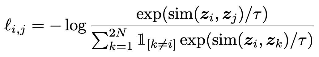
最终的损失是batch中所有正样本对损失的算术平均值:

请记住,在*l(2k- 1,2k) + l(2k, 2k-1)中的索引完全取决于你如何实现损失 —— 我发现当我把它们解释为l(i,j) + l(j, i)*时,更容易理解。
对比损失函数 — PyTorch的实现
如果不先进行矢量化,那么实现损失函数就容易得多,然后再进行矢量化。
import torch
from torch import nn
import torch.nn.functional as F
class ContrastiveLossELI5(nn.Module):
    def __init__(self, batch_size, temperature=0.5, verbose=True):
        super().__init__()
        self.batch_size = batch_size
        self.register_buffer("temperature", torch.tensor(temperature))
        self.verbose = verbose

    def forward(self, emb_i, emb_j):
        """
        emb_i and emb_j are batches of embeddings, where corresponding indices are pairs
        z_i, z_j as per SimCLR paper
        """
        z_i = F.normalize(emb_i, dim=1)
        z_j = F.normalize(emb_j, dim=1)

        representations = torch.cat([z_i, z_j], dim=0)
        similarity_matrix = F.cosine_similarity(representations.unsqueeze(1), representations.unsqueeze(0), dim=2)
        if self.verbose: print("Similarity matrixn", similarity_matrix, "n")

        def l_ij(i, j):
            z_i_, z_j_ = representations[i], representations[j]
            sim_i_j = similarity_matrix[i, j]
            if self.verbose: print(f"sim({i}, {j})={sim_i_j}")

            numerator = torch.exp(sim_i_j / self.temperature)
            one_for_not_i = torch.ones((2 * self.batch_size, )).to(emb_i.device).scatter_(0, torch.tensor([i]), 0.0)
            if self.verbose: print(f"1{{k!={i}}}",one_for_not_i)

            denominator = torch.sum(
                one_for_not_i * torch.exp(similarity_matrix[i, :] / self.temperature)
            )
            if self.verbose: print("Denominator", denominator)

            loss_ij = -torch.log(numerator / denominator)
            if self.verbose: print(f"loss({i},{j})={loss_ij}n")

            return loss_ij.squeeze(0)

        N = self.batch_size
        loss = 0.0
        for k in range(0, N):
            loss += l_ij(k, k + N) + l_ij(k + N, k)
        return 1.0 / (2*N) * loss
解释
对比损失需要知道batch大小和temperature(尺度)参数。你可以在论文中找到设置最佳temperature参数的细节。
我的对比损失的forward的实现中有两个参数。第一个是第一次增强后的图像batch的投影,第二个是第二次增强后的图像batch的投影。
投影首先需要标准化,因此:
z_i = F.normalize(emb_i, dim=1)
z_j = F.normalize(emb_j, dim=1)
所有的表示被拼接在一起,以有效地计算每个图像对之间的余弦相似度。
representations = torch.cat([z_i, z_j], dim=0)
similarity_matrix = F.cosine_similarity(representations.unsqueeze(1), representations.unsqueeze(0), dim=2)
接下来是简单的*l(i,j)*实现,便于理解。下面的代码几乎直接实现了这个等式:

def l_ij(i, j):
    z_i_, z_j_ = representations[i], representations[j]
    sim_i_j = similarity_matrix[i, j]
    numerator = torch.exp(sim_i_j / self.temperature)
    one_for_not_i = torch.ones((2 * self.batch_size, )).to(emb_i.device).scatter_(0, torch.tensor([i]), 0.0)
    denominator = torch.sum(
        one_for_not_i * torch.exp(similarity_matrix[i, :] / self.temperature)
    )

    loss_ij = -torch.log(numerator / denominator)
    return loss_ij.squeeze(0)
然后,该batch的最终损失计算为所有正样本组合的算术平均值:
N = self.batch_size
loss = 0.0
for k in range(0, N):
    loss += l_ij(k, k + N) + l_ij(k + N, k)
return 1.0 / (2*N) * loss
现在,让我们在verbose模式下运行它,看看里面有什么。
I = torch.tensor([[1.0, 2.0], [3.0, -2.0], [1.0, 5.0]])
J = torch.tensor([[1.0, 0.75], [2.8, -1.75], [1.0, 4.7]])
loss_eli5 = ContrastiveLossELI5(batch_size=3, temperature=1.0, verbose=True)
loss_eli5(I, J)
Similarity matrix
    tensor([[ 1.0000, -0.1240,  0.9648,  0.8944, -0.0948,  0.9679],
        [-0.1240,  1.0000, -0.3807,  0.3328,  0.9996, -0.3694],
        [ 0.9648, -0.3807,  1.0000,  0.7452, -0.3534,  0.9999],
        [ 0.8944,  0.3328,  0.7452,  1.0000,  0.3604,  0.7533],
        [-0.0948,  0.9996, -0.3534,  0.3604,  1.0000, -0.3419],
        [ 0.9679, -0.3694,  0.9999,  0.7533, -0.3419,  1.0000]])

sim(0, 3)=0.8944272398948669
1{k!=0} tensor([0., 1., 1., 1., 1., 1.])
Denominator tensor(9.4954)
loss(0,3)=1.3563847541809082

sim(3, 0)=0.8944272398948669
1{k!=3} tensor([1., 1., 1., 0., 1., 1.])
Denominator tensor(9.5058)
loss(3,0)=1.357473373413086

sim(1, 4)=0.9995677471160889
1{k!=1} tensor([1., 0., 1., 1., 1., 1.])
Denominator tensor(6.3699)
loss(1,4)=0.8520082831382751

sim(4, 1)=0.9995677471160889
1{k!=4} tensor([1., 1., 1., 1., 0., 1.])
Denominator tensor(6.4733)
loss(4,1)=0.8681114912033081

sim(2, 5)=0.9999250769615173
1{k!=2} tensor([1., 1., 0., 1., 1., 1.])
Denominator tensor(8.8348)
loss(2,5)=1.1787779331207275

sim(5, 2)=0.9999250769615173
1{k!=5} tensor([1., 1., 1., 1., 1., 0.])
Denominator tensor(8.8762)
loss(5,2)=1.1834462881088257

tensor(1.1327)
这里发生了一些事情,但是通过在冗长的日志和方程之间来回切换,一切都应该变得清楚了。由于相似度矩阵的构造方式,索引按batch大小跳跃,首先是l(0,3), l(3,0),然后是l(1,4), l(4,1)。similarity_matrix的第一行为:
[ 1.0000, -0.1240, 0.9648, 0.8944, -0.0948, 0.9679]
记住这个输入:
I = torch.tensor([[1.0, 2.0], [3.0, -2.0], [1.0, 5.0]])
J = torch.tensor([[1.0, 0.75], [2.8, -1.75], [1.0, 4.7]])
现在:
1.0000 是 I[0] and I[0]([1.0, 2.0] and [1.0, 2.0]) 之间的余弦相似度
-0.1240是I[0] and I[1] ([1.0, 2.0] and [3.0, -2.0])之间的余弦相似度
-0.0948是I[0] and J[2] ([1.0, 2.0] and [2.8, -1.75])之间的余弦相似度
等等
第一次的图像投影之间的相似性越高,损失越小:
I = torch.tensor([[1.0, 2.0], [3.0, -2.0], [1.0, 5.0]])
J = torch.tensor([[1.0, 0.75], [2.8, -1.75], [1.0, 4.7]])
J = torch.tensor([[1.0, 1.75], [2.8, -1.75], [1.0, 4.7]]) # note the change
ContrastiveLossELI5(3, 1.0, verbose=False)(I, J)
tensor(1.0996)
的确,损失减少了!现在我将继续介绍向量化的实现。
对比损失函数 — PyTorch的实现,向量版本
朴素的实现的性能真的很差(主要是由于手动循环),看看结果:
contrastive_loss_eli5 = ContrastiveLossELI5(3, 1.0, verbose=False)
I = torch.tensor([[1.0, 2.0], [3.0, -2.0], [1.0, 5.0]], requires_grad=True)
J = torch.tensor([[1.0, 0.75], [2.8, -1.75], [1.0, 4.7]], requires_grad=True)
%%timeit
contrastive_loss_eli5(I, J)
838 µs ± 23.8 µs per loop (mean ± std. dev. of 7 runs, 1000 loops each)
一旦我理解了损失的内在,就很容易对其进行向量化并去掉手动循环:
class ContrastiveLoss(nn.Module):
    def __init__(self, batch_size, temperature=0.5):
        super().__init__()
        self.batch_size = batch_size
        self.register_buffer("temperature", torch.tensor(temperature))
        self.register_buffer("negatives_mask", (~torch.eye(batch_size * 2, batch_size * 2, dtype=bool)).float())

    def forward(self, emb_i, emb_j):
        """
        emb_i and emb_j are batches of embeddings, where corresponding indices are pairs
        z_i, z_j as per SimCLR paper
        """
        z_i = F.normalize(emb_i, dim=1)
        z_j = F.normalize(emb_j, dim=1)

        representations = torch.cat([z_i, z_j], dim=0)
        similarity_matrix = F.cosine_similarity(representations.unsqueeze(1), representations.unsqueeze(0), dim=2)

        sim_ij = torch.diag(similarity_matrix, self.batch_size)
        sim_ji = torch.diag(similarity_matrix, -self.batch_size)
        positives = torch.cat([sim_ij, sim_ji], dim=0)

        nominator = torch.exp(positives / self.temperature)
        denominator = self.negatives_mask * torch.exp(similarity_matrix / self.temperature)

        loss_partial = -torch.log(nominator / torch.sum(denominator, dim=1))
        loss = torch.sum(loss_partial) / (2 * self.batch_size)
        return loss
contrastive_loss = ContrastiveLoss(3, 1.0)
contrastive_loss(I, J).item() - contrastive_loss_eli5(I, J).item()
0.0
差应为零或接近零,性能比较:
I = torch.tensor([[1.0, 2.0], [3.0, -2.0], [1.0, 5.0]], requires_grad=True)
J = torch.tensor([[1.0, 0.75], [2.8, -1.75], [1.0, 4.7]], requires_grad=True)
%%timeit
contrastive_loss_eli5(I, J)
918 µs ± 60.2 µs per loop (mean ± std. dev. of 7 runs, 1000 loops each)
%%timeit
contrastive_loss(I, J)
272 µs ± 9.18 µs per loop (mean ± std. dev. of 7 runs, 1000 loops each)
几乎是4倍的提升,非常有效。
使用SimCLR和EfficientNet预训练图像嵌入
一旦建立并理解了损失函数,就是时候好好利用它了。我将使用EfficientNet架构,按照SimCLR框架对图像嵌入进行预训练。为了方便起见,我实现了几个实用函数和类,我将在下面简要解释它们。训练代码使用PyTorch-Lightning构造。
我使用了EfficientNet,在ImageNet上进行了预训练,我选择的数据集是STL10,包含了训练和未标记的分割,用于无监督/自监督学习任务。
我在这里的目标是演示整个SimCLR流程。我并不是要使用当前的配置获得新的SOTA。
图像增强函数
使用SimCLR进行训练可以生成良好的图像嵌入,而不会受到图像变换的影响 —— 这是因为在训练期间,进行了各种数据增强,以迫使网络理解图像的内容,而不考虑图像的颜色或图像中物体的位置。SimCLR的作者说,数据增强的组成在定义有效的预测任务中扮演着关键的角色,而且对比学习需要比监督学习更强的数据增强。综上所述:在对图像嵌入进行预训练时,最好通过对图像进行强增强,使网络学习变得困难一些,以便以后更好地进行泛化。
我强烈建议阅读SimCLR的论文和附录,因为他们做了消融研究,数据增加对嵌入带来最好的效果。
为了让这篇博文更简单,我将主要使用内置的Torchvision数据增强功能,还有一个额外功能 —— 随机调整缩放旋转。
def random_rotate(image):
    if random.random() > 0.5:
        return tvf.rotate(image, angle=random.choice((0, 90, 180, 270)))
    return image
class ResizedRotation():
    def __init__(self, angle, output_size=(96, 96)):
        self.angle = angle
        self.output_size = output_size

    def angle_to_rad(self, ang): return np.pi * ang / 180.0

    def __call__(self, image):
        w, h = image.size
        new_h = int(np.abs(w * np.sin(self.angle_to_rad(90 - self.angle))) + np.abs(h * np.sin(self.angle_to_rad(self.angle))))
        new_w = int(np.abs(h * np.sin(self.angle_to_rad(90 - self.angle))) + np.abs(w * np.sin(self.angle_to_rad(self.angle))))
        img = tvf.resize(image, (new_w, new_h))
        img = tvf.rotate(img, self.angle)
        img = tvf.center_crop(img, self.output_size)
        return img
class WrapWithRandomParams():
    def __init__(self, constructor, ranges):
        self.constructor = constructor
        self.ranges = ranges

    def __call__(self, image):
        randoms = [float(np.random.uniform(low, high)) for _, (low, high) in zip(range(len(self.ranges)), self.ranges)]
        return self.constructor(*randoms)(image)

from torchvision.datasets import STL10
import torchvision.transforms.functional as tvf
from torchvision import transforms
import numpy as np
简单看一下变换结果:
stl10_unlabeled = STL10(".", split="unlabeled", download=True)
idx = 123
random_resized_rotation = WrapWithRandomParams(lambda angle: ResizedRotation(angle), [(0.0, 360.0)])
random_resized_rotation(tvf.resize(stl10_unlabeled[idx][0], (96, 96)))
自动数据增强wrApper
在这里,我还实现了一个dataset wrapper,它在每次检索图像时自动应用随机数据扩充。它可以很容易地与任何图像数据集一起使用,只要它遵循简单的接口返回 tuple ,(PIL Image, anything)。当把debug 标志设置为True,可以将这个wrapper设置为返回一个确定性转换。请注意,有一个preprocess步骤,应用ImageNet的数据标准化,因为我使用的是预训练好的EfficientNet。
from torch.utils.data import Dataset, DataLoader, SubsetRandomSampler, SequentialSampler
import random
class PretrainingDatasetWrapper(Dataset):
    def __init__(self, ds: Dataset, target_size=(96, 96), debug=False):
        super().__init__()
        self.ds = ds
        self.debug = debug
        self.target_size = target_size
        if debug:
            print("DATASET IN DEBUG MODE")

        # I will be using network pre-trained on ImageNet first, which uses this normalization.
        # Remove this, if you're training from scratch or apply different transformations accordingly
        self.preprocess = transforms.Compose([
                transforms.ToTensor(),
                transforms.Normalize(mean=[0.485, 0.456, 0.406], std=[0.229, 0.224, 0.225]),
        ])

        random_resized_rotation = WrapWithRandomParams(lambda angle: ResizedRotation(angle, target_size), [(0.0, 360.0)])
        self.randomize = transforms.Compose([
            transforms.RandomResizedCrop(target_size, scale=(1/3, 1.0), ratio=(0.3, 2.0)),
            transforms.RandomChoice([
                transforms.RandomHorizontalFlip(p=0.5),
                transforms.Lambda(random_rotate)
            ]),
            transforms.RandomApply([
                random_resized_rotation
            ], p=0.33),
            transforms.RandomApply([
                transforms.ColorJitter(brightness=0.5, contrast=0.5, saturation=0.5, hue=0.2)
            ], p=0.8),
            transforms.RandomGrayscale(p=0.2)
        ])

    def __len__(self): return len(self.ds)

    def __getitem_internal__(self, idx, preprocess=True):
        this_image_raw, _ = self.ds[idx]

        if self.debug:
            random.seed(idx)
            t1 = self.randomize(this_image_raw)
            random.seed(idx + 1)
            t2 = self.randomize(this_image_raw)
        else:
            t1 = self.randomize(this_image_raw)
            t2 = self.randomize(this_image_raw)

        if preprocess:
            t1 = self.preprocess(t1)
            t2 = self.preprocess(t2)
        else:
            t1 = transforms.ToTensor()(t1)
            t2 = transforms.ToTensor()(t2)

        return (t1, t2), torch.tensor(0)

    def __getitem__(self, idx):
        return self.__getitem_internal__(idx, True)

    def raw(self, idx):
        return self.__getitem_internal__(idx, False)
ds = PretrainingDatasetWrapper(stl10_unlabeled, debug=False)
tvf.to_pil_image(ds[idx][0][0])
tvf.to_pil_image(ds[idx][0][1])
tvf.to_pil_image(ds.raw(idx)[0][1])
tvf.to_pil_image(ds.raw(idx)[0][0])
SimCLR神经网络生成嵌入
这里我定义了基于EfficientNet-b0架构的ImageEmbedding神经网络。我用identity函数替换了EfficientNet 的最后一层,在它的上面(跟在SimCLR的后面)添加了Linear-ReLU-Linear 层得到图像嵌入。本文表明,非线性投影头,也就是Linear-ReLU-Linear提高嵌入的质量。
from efficientnet_pytorch import EfficientNet
class ImageEmbedding(nn.Module):
    class Identity(nn.Module):
        def __init__(self): super().__init__()

        def forward(self, x):
            return x


    def __init__(self, embedding_size=1024):
        super().__init__()

        base_model = EfficientNet.from_pretrained("efficientnet-b0")
        internal_embedding_size = base_model._fc.in_features
        base_model._fc = ImageEmbedding.Identity()

        self.embedding = base_model

        self.projection = nn.Sequential(
            nn.Linear(in_features=internal_embedding_size, out_features=embedding_size),
            nn.ReLU(),
            nn.Linear(in_features=embedding_size, out_features=embedding_size)
        )

    def calculate_embedding(self, image):
        return self.embedding(image)

    def forward(self, X):
        image = X
        embedding = self.calculate_embedding(image)
        projection = self.projection(embedding)
        return embedding, projection
接下来是基于PyTorch-Lightning的训练模块的实现,它将所有的事情协调在一起:
- 超参数处理
- SimCLR图像嵌入网络
- STL10数据集
- 优化器
- 前向步骤
在PretrainingDatasetWrapper中,我实现了返回元组:(Image1, Image2), dummy class,这个模块的前向步骤是很简单的,它需要产生两个batch的嵌入和计算对比损失函数:
(X, Y), y = batch
embX, projectionX = self.forward(X)
embY, projectionY = self.forward(Y)
loss = self.loss(projectionX, projectionY)
from torch.multiprocessing import cpu_count
from torch.optim import RMSprop
import pytorch_lightning as pl
class ImageEmbeddingModule(pl.LightningModule):
    def __init__(self, hparams):
        hparams = Namespace(**hparams) if isinstance(hparams, dict) else hparams
        super().__init__()
        self.hparams = hparams
        self.model = ImageEmbedding()
        self.loss = ContrastiveLoss(hparams.batch_size)

    def total_steps(self):
        return len(self.train_dataloader()) // self.hparams.epochs

    def train_dataloader(self):
        return DataLoader(PretrainingDatasetWrapper(stl10_unlabeled,
                                             debug=getattr(self.hparams, "debug", False)),
                          batch_size=self.hparams.batch_size,
                          num_workers=cpu_count(),
                          sampler=SubsetRandomSampler(list(range(hparams.train_size))),
                         drop_last=True)

    def val_dataloader(self):
        return DataLoader(PretrainingDatasetWrapper(stl10_unlabeled,
                                            debug=getattr(self.hparams, "debug", False)),
                          batch_size=self.hparams.batch_size,
                          shuffle=False,
                          num_workers=cpu_count(),
                          sampler=SequentialSampler(list(range(hparams.train_size + 1, hparams.train_size + hparams.validation_size))),
                         drop_last=True)

    def forward(self, X):
        return self.model(X)

    def step(self, batch, step_name = "train"):
        (X, Y), y = batch
        embX, projectionX = self.forward(X)
        embY, projectionY = self.forward(Y)
        loss = self.loss(projectionX, projectionY)
        loss_key = f"{step_name}_loss"
        tensorboard_logs = {loss_key: loss}

        return { ("loss" if step_name == "train" else loss_key): loss, 'log': tensorboard_logs,
                        "progress_bar": {loss_key: loss}}

    def training_step(self, batch, batch_idx):
        return self.step(batch, "train")

    def validation_step(self, batch, batch_idx):
        return self.step(batch, "val")

    def validation_end(self, outputs):
        if len(outputs) == 0:
            return {"val_loss": torch.tensor(0)}
        else:
            loss = torch.stack([x["val_loss"] for x in outputs]).mean()
            return {"val_loss": loss, "log": {"val_loss": loss}}

    def configure_optimizers(self):
        optimizer = RMSprop(self.model.parameters(), lr=self.hparams.lr)
        return [optimizer], []
超参数初始化。Batch size大小为128,在GTX1070上使用EfficientNet-B0运行的很好。注意,为了方便以Jupyter Notebook /google Colab的形式运行这篇博客文章,我将训练数据集限制为STL10的前10k图像。
重要!SimCLR从大Batch size中得到了极大的好处 —— 它应该在GPU/集群限制下被设置为尽可能高。
from argparse import Namespace
hparams = Namespace(
    lr=1e-3,
    epochs=50,
    batch_size=160,
    train_size=10000,
    validation_size=1000
)
使用LRFinder算法寻找好的初始学习率
我使用pytorch-lightning的内置LRFinder算法来查找初始学习率。
module = ImageEmbeddingModule(hparams)
t = pl.Trainer(gpus=1)
lr_finder = t.lr_find(module)
GPU available: True, used: True
TPU available: False, using: 0 TPU cores
CUDA_VISIBLE_DEVICES: [0]

   | Name  | Type            | Params
------------------------------------------
0 | model | ImageEmbedding  | 6 M
1 | loss  | ContrastiveLoss | 0
lr_finder.plot(show=False, suggest=True)
lr_finder.suggestion()
0.000630957344480193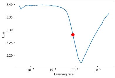
我也使用W&B日志记录我的实验:
from pytorch_lightning.loggers import WandbLogger
hparams = Namespace(
    lr=0.000630957344480193,
    epochs=10,
    batch_size=160,
    train_size=20000,
    validation_size=1000
)
module = ImageEmbeddingModule(hparams)
logger = WandbLogger(project="simclr-blogpost")
logger.watch(module, log="all", log_freq=50)
trainer = pl.Trainer(gpus=1, logger=logger)
trainer.fit(module)
| Name  | Type            | Params
------------------------------------------
0 | model | ImageEmbedding  | 6 M
1 | loss  | ContrastiveLoss | 0
训练完成后,图像嵌入就可以用于下游任务了。
在SimCLR嵌入上进行图像分类
一旦训练好嵌入,它们就可以用来训练在它们之上的分类器 —— 可以通过微调整个网络,也可以通过用嵌入冻结基础网络并在其之上学习线性分类器 ——下面我将展示后者。
使用嵌入保存神经网络的权值
我以检查点的形式保存整个网络。之后,只有网络的内部部分将与分类器一起使用(投影层将被丢弃)。
checkpoint_file = "efficientnet-b0-stl10-embeddings.ckpt"
trainer.save_checkpoint(checkpoint_file)
trainer.logger.experiment.log_artifact(checkpoint_file, type="model")
分类器模块
同样,我定义了一个自定义模块 —— 这次它使用了已经存在的嵌入并根据需要冻结了基础模型的权重。注意SimCLRClassifier.embeddings只是整个网络之前使用的EfficientNet的一部分 —— 投影头被丢弃。
class SimCLRClassifier(nn.Module):
    def __init__(self, n_classes, freeze_base, embeddings_model_path, hidden_size=512):
        super().__init__()

        base_model = ImageEmbeddingModule.load_from_checkpoint(embeddings_model_path).model

        self.embeddings = base_model.embedding

        if freeze_base:
            print("Freezing embeddings")
            for param in self.embeddings.parameters():
                param.requires_grad = False

        # Only linear projection on top of the embeddings should be enough
        self.classifier = nn.Linear(in_features=base_model.projection[0].in_features,
                      out_features=n_classes if n_classes > 2 else 1)


    def forward(self, X, *args):
        emb = self.embeddings(X)
        return self.classifier(emb)
分类器训练代码
分类器训练代码再次使用PyTorch lightning,所以我跳过了深入的解释。
from torch import nn
from torch.optim.lr_scheduler import CosineAnnealingLR
class SimCLRClassifierModule(pl.LightningModule):
    def __init__(self, hparams):
        super().__init__()
        hparams = Namespace(**hparams) if isinstance(hparams, dict) else hparams
        self.hparams = hparams
        self.model = SimCLRClassifier(hparams.n_classes, hparams.freeze_base,
                                      hparams.embeddings_path,
                                      self.hparams.hidden_size)
        self.loss = nn.CrossEntropyLoss()

    def total_steps(self):
        return len(self.train_dataloader()) // self.hparams.epochs

    def preprocessing(seff):
        return transforms.Compose([
                transforms.ToTensor(),
                transforms.Normalize(mean=[0.485, 0.456, 0.406], std=[0.229, 0.224, 0.225]),
        ])

    def get_dataloader(self, split):
        return DataLoader(STL10(".", split=split, transform=self.preprocessing()),
                          batch_size=self.hparams.batch_size,
                          shuffle=split=="train",
                          num_workers=cpu_count(),
                         drop_last=False)

    def train_dataloader(self):
        return self.get_dataloader("train")

    def val_dataloader(self):
        return self.get_dataloader("test")

    def forward(self, X):
        return self.model(X)

    def step(self, batch, step_name = "train"):
        X, y = batch
        y_out = self.forward(X)
        loss = self.loss(y_out, y)
        loss_key = f"{step_name}_loss"
        tensorboard_logs = {loss_key: loss}

        return { ("loss" if step_name == "train" else loss_key): loss, 'log': tensorboard_logs,
                        "progress_bar": {loss_key: loss}}

    def training_step(self, batch, batch_idx):
        return self.step(batch, "train")

    def validation_step(self, batch, batch_idx):
        return self.step(batch, "val")

    def test_step(self, batch, batch_idx):
        return self.step(Batch, "test")

    def validation_end(self, outputs):
        if len(outputs) == 0:
            return {"val_loss": torch.tensor(0)}
        else:
            loss = torch.stack([x["val_loss"] for x in outputs]).mean()
            return {"val_loss": loss, "log": {"val_loss": loss}}

    def configure_optimizers(self):
        optimizer = RMSprop(self.model.parameters(), lr=self.hparams.lr)
        schedulers = [
            CosineAnnealingLR(optimizer, self.hparams.epochs)
        ] if self.hparams.epochs > 1 else []
        return [optimizer], schedulers
这里值得一提的是,使用frozen的基础模型进行训练可以在训练过程中极大地提高性能,因为只需要计算单个层的梯度。此外,利用良好的嵌入,只需几个epoch就能得到高质量的单线性投影分类器。
hparams_cls = Namespace(
    lr=1e-3,
    epochs=5,
    batch_size=160,
    n_classes=10,
    freeze_base=True,
    embeddings_path="./efficientnet-b0-stl10-embeddings.ckpt",
    hidden_size=512
)
module = SimCLRClassifierModule(hparams_cls)
logger = WandbLogger(project="simclr-blogpost-classifier")
logger.watch(module, log="all", log_freq=10)
trainer = pl.Trainer(gpus=1, max_epochs=hparams_cls.epochs, logger=logger)
lr_find_cls = trainer.lr_find(module)
| Name  | Type             | Params
-------------------------------------------
0 | model | SimCLRClassifier | 4 M
1 | loss  | CrossEntropyLoss | 0
LR finder stopped early due to diverging loss.
lr_find_cls.plot(show=False, suggest=True)
lr_find_cls.suggestion()
0.003981071705534969
hparams_cls = Namespace(
    lr=0.003981071705534969,
    epochs=5,
    batch_size=160,
    n_classes=10,
    freeze_base=True,
    embeddings_path="./efficientnet-b0-stl10-embeddings.ckpt",
    hidden_size=512
)
module = SimCLRClassifierModule(hparams_cls)
trainer.fit(module)
| Name  | Type             | Params
-------------------------------------------
0 | model | SimCLRClassifier | 4 M
1 | loss  | CrossEntropyLoss | 0
评估
这里我定义了一个utility函数,用来评估模型。注意,对于大的数据集,在GPU和CPU之间的传输和存储所有的结果在内存中是不可能的。
from sklearn.metrics import classification_report
def evaluate(data_loader, module):
    with torch.no_grad():
        progress = ["/", "-", "\", "|", "/", "-", "\", "|"]
        module.eval().cuda()
        true_y, pred_y = [], []
        for i, batch_ in enumerate(data_loader):
            X, y = batch_
            print(progress[i % len(progress)], end="r")
            y_pred = torch.argmax(module(X.cuda()), dim=1)
            true_y.extend(y.cpu())
            pred_y.extend(y_pred.cpu())
        print(classification_report(true_y, pred_y, digits=3))
        return true_y, pred_y
_ = evaluate(module.val_dataloader(), module)
                  precision    recall  f1-score   support

               0      0.856     0.864     0.860       800
               1      0.714     0.701     0.707       800
               2      0.903     0.919     0.911       800
               3      0.678     0.599     0.636       800
               4      0.665     0.746     0.703       800
               5      0.633     0.564     0.597       800
               6      0.729     0.781     0.754       800
               7      0.678     0.709     0.693       800
               8      0.868     0.910     0.888       800
               9      0.862     0.801     0.830       800

        accuracy                          0.759      8000
       macro avg      0.759     0.759     0.758      8000
    weighted avg      0.759     0.759     0.758      8000
总结
我希望我对SimCLR框架的解释对你有所帮助。
英文原文:https://zablo.net/blog/post/understanding-implementing-simclr-guide-eli5-pytorch/